By Efraim Berkovich
PWBM’s Dynamic OLG model simulates the partially-open U.S. economy in a way that is more consistent with economic behavior than standard “model blending” exercises. The difference between the two techniques becomes more pronounced over time due to the nation’s expanding debt path.
Background
The openness of the U.S. economy to foreign capital flows helps determine the path of capital growth and, thus, future GDP. If the U.S. economy were completely closed to capital flows, all government debt and productive capital would be owned, by definition, by U.S. households. In this scenario, new debt crowds out productive investment, reducing GDP.
Opening the economy implies that foreigners purchase some of capital and debt, thereby reducing crowd-out. If the United States were both a small country and fully open to international capital flow (also known as a “small open economy”), debt would have no effect on capital formation. In reality, the United States is both large and not fully open. The U.S. economy, therefore, is best described as “partially open,” where foreign flows exist but are not at the level of a fully open economy.
Two Approaches: PWBM vs. Standard “Model Blending”
PWBM's Dynamic OLG model allows for partial foreign flows on a time-varying basis (to model policies that might impact the openness over time). An alternative and fairly standard approach would be to estimate a partially-open economy through a convex combination of solutions for a closed economy and a fully open economy, which is standard with “model blending” exercises. This alternative is less costly in terms of calculations. However, under this approach, forward-looking agents are not fully aware of the restrictions on capital flows.1 Awareness of those restrictions may influence decisions to work and save, thereby affecting projections of labor, capital and GDP. Moreover, there is no reason to expect consistency between GDP as calculated from the nonlinear Cobb-Douglas production function and the inputs of capital and labor in the alternative convex estimate.
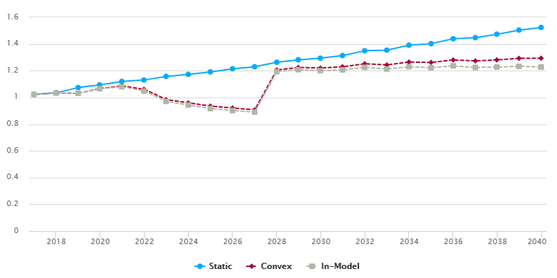
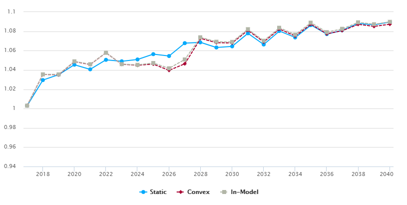
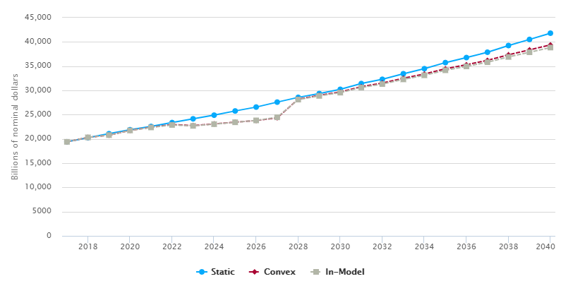
PWBM has previous documented the government’s expanding debt path under current law (see Figure 3 here). Below, Figures 1 to 3 display PWBM’s projections for future capital, labor and GDP under three scenarios. The “in-model” dynamic approach corresponds to PWBM’s modeling of how changes in debt influence the economy over time. The “convex” dynamic projection corresponds to the alternative, simpler method described above for incorporating debt effects. In each case, the economy is assumed to be permanently 40 percent open (in both debt and capital).2 As a comparison, the “static” projection is shown that corresponds to conventional forecasts often used in policy analysis that do not allow GDP and capital to change in response to fiscal policy, including a growing debt over time.
Notice that the “in-model” and “convex” approaches are fairly close for the first 10 years. Kinks in early years are due to expiring provisions in the Tax Cuts and Jobs Act, especially related to changes to the tax treatment of investment. However, in the long-run, the differences widen. By 2040, PWBM’s in-model capital is 5.1 percent lower compared to the alternative convex estimate, which pulls GDP down by 1.4 percent relative to the convex approach. The reason is that households in the in-model approach correctly fully incorporate the steep rising debt path, which is only approximated by the convex approach.
As such, PWBM’s modeling approach applies a useful enhancement to common “model blending” methods. PWBM’s approach is especially important with growing debt paths.
-
In more technical terms, the difference follows Jensen’s Inequality. Convexification works well at modest second derivatives but becomes less accurate as the second derivative increases in value. As an example, see the figure here. ↩
-
Consistent with our previous dynamic analysis and the empirical evidence, our baseline assumes that the U.S. economy is 40 percent open and 60 percent closed. Specifically, 40 percent of new government debt is purchased by foreigners. ↩
  Year,Static,Convex,In-Model
  2017,1.022448941,1.022448941,1.022448941
  2018,1.034979173,1.032189042,1.032720238
  2019,1.073919301,1.03061762,1.031121098
  2020,1.09337552,1.066759105,1.064987923
  2021,1.120000807,1.085878385,1.08014423
  2022,1.130783306,1.060692242,1.048042232
  2023,1.15776592,0.983801929,0.970699598
  2024,1.172606009,0.959533144,0.943450602
  2025,1.191453665,0.935016476,0.917027987
  2026,1.214795342,0.920629791,0.901860143
  2027,1.229857816,0.907399649,0.890233193
  2028,1.263184743,1.205569269,1.193170987
  2029,1.282154246,1.224478472,1.208102441
  2030,1.293990261,1.220063473,1.200499515
  2031,1.313906491,1.229835711,1.206644163
  2032,1.349565917,1.252204425,1.224847799
  2033,1.354087894,1.243557477,1.212810356
  2034,1.391383441,1.265054217,1.229874437
  2035,1.402545444,1.261882805,1.222554194
  2036,1.439479676,1.280707995,1.236315361
  2037,1.447533076,1.273338647,1.224618731
  2038,1.473563438,1.281304442,1.227382149
  2039,1.504474302,1.292705784,1.232766489
  2040,1.52380527,1.293403821,1.227497001
  Year,Static,Convex,In-Model
  2017,1.002987998,1.002987998,1.002987998
  2018,1.029490661,1.035305914,1.035412054
  2019,1.035112682,1.034990668,1.035388953
  2020,1.045406082,1.048614361,1.048885042
  2021,1.040625534,1.045601606,1.045902414
  2022,1.050471452,1.057794626,1.057806405
  2023,1.048972279,1.045871471,1.046029951
  2024,1.050842082,1.044897533,1.045264249
  2025,1.056359689,1.046035035,1.047153413
  2026,1.054416056,1.039585221,1.041669511
  2027,1.067756883,1.046380615,1.050854619
  2028,1.06854837,1.072649497,1.073781382
  2029,1.063244933,1.068229822,1.069175385
  2030,1.064425268,1.067939275,1.069002391
  2031,1.07793661,1.081064365,1.08216952
  2032,1.066336755,1.068998919,1.070173966
  2033,1.080295973,1.082340801,1.08366049
  2034,1.073646398,1.075121091,1.076545339
  2035,1.086421296,1.087350784,1.088904448
  2036,1.077133745,1.077410891,1.079098669
  2037,1.081081352,1.080728548,1.082577861
  2038,1.088235066,1.087230385,1.089285138
  2039,1.086715386,1.08509622,1.087309141
  2040,1.089615661,1.087353581,1.089798903
  Year,Static,Convex,In-Model
  2017,19390.605,19390.605,19390.605
  2018,20247.15208,20303.8146,20308.84245
  2019,21071.91739,20774.781,20786.22065
  2020,21886.70587,21746.74496,21739.43804
  2021,22566.13098,22398.22193,22364.36253
  2022,23363.6766,22956.859,22872.59604
  2023,24134.76401,22740.14256,22689.02431
  2024,24890.28836,23084.07122,23035.47653
  2025,25756.13379,23446.25659,23426.93652
  2026,26560.59686,23784.83623,23810.46997
  2027,27582.29301,24344.54612,24453.29864
  2028,28564.21803,28180.00494,28106.25113
  2029,29350.40459,28978.24248,28868.48128
  2030,30218.84506,29675.95675,29541.6182
  2031,31414.10957,30762.96579,30596.59579
  2032,32287.66955,31512.90053,31314.7026
  2033,33435.30346,32501.97654,32272.02878
  2034,34474.38032,33381.60107,33116.93518
  2035,35729.52787,34455.93453,34150.81049
  2036,36766.84981,35300.51745,34955.28918
  2037,37870.67512,36197.91165,35810.14488
  2038,39248.3688,37342.72218,36906.75436
  2039,40505.02051,38356.90588,37866.40282
  2040,41797.63644,39388.22328,38839.24656