Summary

The financial condition of Social Security is worsening at a much faster rate than official estimates. A balanced reform, combining progressive benefit cuts and tax increases, produces the strongest economic growth relative to plausible options that only rely on benefit cuts or tax increases.

Key Points

We examine a range of policy options that put Social Security on a sustainable path.
The analysis emphasizes the need for analyzing Social Security reforms using deep modeling that reveals important interactions that challenge conventional wisdom.
Tax increases generally produce more growth than “current policy” analysis where shortfalls are combined with the standard unified surplus measure. Additional debt can be combined with changes in benefits to produce even more economic growth. Reforms that combine tax increases and progressive benefit reductions produce the most growth.

Options to Return Social Security to Financial Balance: The Impact on Economic Growth

Introduction

In 2018, more than 52 million people received retirement benefits from Social Security, a figure that will rise as more baby boomers claim benefits. Our previous analysis shows that Social Security’s financial condition is worsening much faster than projections provided by the Social Security Trustees Reports. The Penn Wharton Budget Model (PWBM) platform provides sometimes counterintuitive but deeper insights into the mechanics of Social Security baseline policy and reform options. The PWBM platform also addresses a common but important inconsistency that arises from mixing “current law” and “current policy” concepts.

In this brief, we examine six potential options to put Social Security on a sustainable path. These reform options are merely illustrative rather than suggestive, as PWBM does not make policy recommendations. Hundreds of other reform option combinations can be explored on our Social Security Simulator. This brief focuses on explaining the macro-economic considerations of Social Security reform; future briefs will consider distributional and other effects.

Short Primer on Social Security Analysis: Understanding Labor Supply Distortions

Social Security benefits are directly tied to earnings through a progressive formula that converts past earnings into benefits. For a worker who retires today, each year of her past taxable wage is adjusted upward by a “wage indexed factor” that gives the worker the value of general economic growth (technically, the growth of taxable earnings) that occurred since that past wage was earned. The worker’s best 35 years of wage-indexed earnings are selected and averaged to create an Average Index of Monthly Earnings (AIME). For workers who retired in 2018, initial benefits at retirement are calculated progressively to replace 90 percent of the first $895 of AIME, 32 percent of AIME between $895 and $5,397, and 15 percent of AIME above $5,397. These dollar thresholds are wage indexed each year. Wage indexation of past taxable wages allows initial benefits to maintain a comparable standard of living relative to younger people. Subsequent benefits, after retirement, are adjusted upward at the inflation rate.

The marginal link between wages and benefits means that Social Security is fundamentally different than other government spending. For most government programs, there is no marginal linkage between the taxes someone pays and benefits received (e.g. military protection). As a result, taxes that fund these other programs generally cause taxpayers to distort their behavior to reduce their tax bills. Common distortions include reducing labor supply, reclassifying income to a different business entity form with a lower tax rate, and deferring income realization. Moreover, the economic distortions associated with these taxes increases by the square of the tax rate, meaning that a doubling of taxes can cause these distortions to increase by four times.

Social Security payroll taxes, however, operate differently since payroll taxes paid into the system are tied closely to future benefits earned, with a few notable exceptions.1 To conceptually understand the importance of the Social Security marginal tax-benefit linkage, suppose that (i) the economy (technically, the Social Security taxable payroll) grows at the same rate as the government’s borrowing rate. Moreover, suppose that (ii) monthly benefits are not progressive so that everyone received the same flat percent replacement of their AIME, for example, 50% of their AIME. Under these conditions, every dollar contributed to Social Security today generates one dollar in present value of future benefits. Social Security taxes, therefore, would not cause households to reduce their labor supply, except for households with no personal savings who would like to borrow against future income. Of course, neither condition (i) or (ii) holds in practice and so payroll taxes produce some economic distortion. Still, the important role of the marginal linkage is useful for understanding why the “donut hole’’ tax, discussed below, generally causes much more labor supply distortion than reforms that simply increase the existing payroll tax rate. Unlike an increase in payroll taxes, this “donut hole” tax is not associated with larger benefits.

Short Primer on Social Security Analysis: Understanding the Baseline

Our analysis is done relative to the “current policy” baseline, which assumes that annual shortfalls are part of the unified surplus. The experts at the Congressional Budget Office (CBO) make a similar assumption. In contrast, under the alternative “current law” baseline, benefits would be cut across the board upon depletion of the trust fund. Social Security, therefore, never faces any financial shortfall under the current law baseline. In expressing actuarial deficits, the Social Security Trustees regularly divide current policy deficits by the current law taxable payroll base. In their 2018 Report, for example, the Trustees report a 75-year actuarial deficit of 2.84 percent of taxable payroll. This number is widely misinterpreted to mean that Social Security could be put on a solvent path for 75 years if payroll taxes were increased immediately and permanently by 2.84 percentage points. However, that interpretation is generally incorrect because, with economic distortions associated with a tax or dynamic effects with debt, the current policy taxable payroll is smaller than the current law tax base. We have previously shown that Social Security is in much worse shape relative to current policy.

Options to Restore Financial Balance

Table 1 presents six different options for restoring financial balance to Social Security: Options A, B, C, D, E and F. Generally speaking, options on the leftward side of Table 1 achieve financial balance by raising taxes while options on the rightward side of Table 1 achieve financial balance by reducing benefits.

Table 1: Social Security Provision Options to Restore Financial Balance

DOWNLOAD DATA

		Option (Current Policy in Red)
	Current Policy	A	B	C	D	E	F
Tax Provision
OASDI Tax Rate	12.4%	14.9%	14.9%	Progressive Increase2	13.6%	13.6%	12.4%
Taxable Maximum3	$128,700	$128,700	$150,000	$128,700	$150,000	$150,000	$128,700
Payroll Taxes on Wage Earnings Above $250,000 ("Donut-Hole")4	None	Full OASDI Rate	1/2 OASDI Rate	Full OASDI Rate	1/2 OASDI Rate	None	None
Benefit Provision
Cost of Living Adjustment (COLA) Index5	CPI	CPI	CPI	CPI-E6	Chained CPI7	Chained CPI8	Chained CPI9
Primary Insurance Amount (PIA)10	90/30/15	90/30/15	90/30/15	90/25/8	90/25/8	90/25/8	80/22/5
Full-Benefit Retirement Age (FRA)11	67	67	68	67	68	70	70

Note: Consistent with our previous dynamic analysis and the empirical evidence, the projections above assume that the U.S. economy is 40 percent open and 60 percent closed. Specifically, 40 percent of new government debt is purchased by foreigners.

Comparison of Options

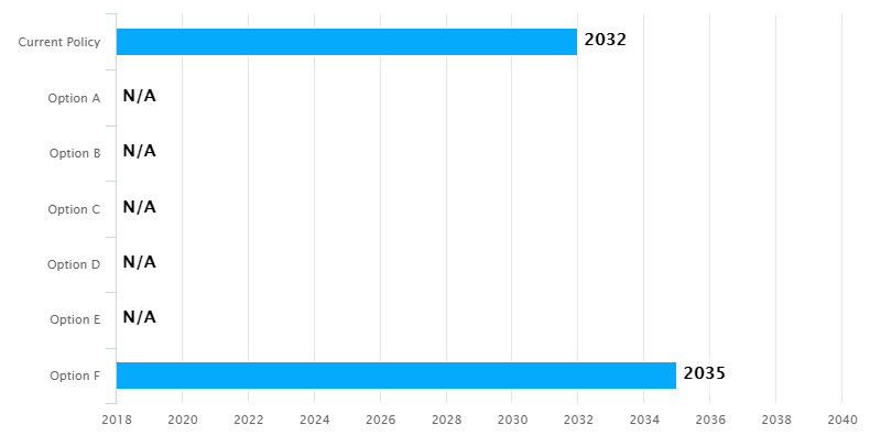
Under current policy, Social Security’s trust fund is depleted in 2032. As seen in Figure 1, the trust fund retains a positive balance under five of the six options examined. Although Option F achieves long-run balance, the Social Security’s trust fund is still depleted in 2035, just three years later than under the current policy baseline scenario. Under the “current policy” scenario, shortfalls in Option F become part of the government’s unified surplus/deficit, implying that additional debt would be issued to cover payable benefits. As noted earlier, under the alternative “current law” baseline, Social Security never faces a solvency problem, by construction.

Figure 1: Social Security Trust Fund Depletion Date

DOWNLOAD DATA

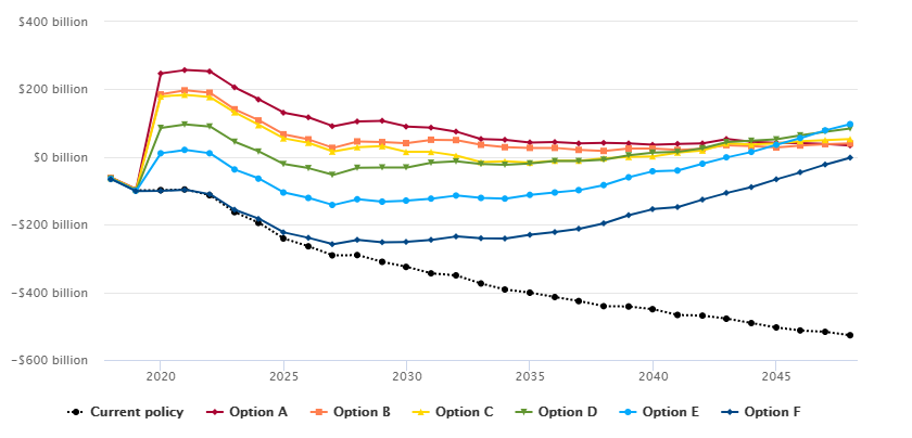
Figure 2 shows the effect of current policy and each of the six options on Social Security’s annual non-interest income balance.12 This measure equals the tax revenue from Social Security taxes less the benefits paid. The black line shows that under current policy there is a negative cash flow that increases as time passes. Notice that options that rely more on tax increases (red, orange and yellow lines) provide a short-run boost to the non-interest measure that flattens out over time. In contrast, options that reduce benefits over time provide a smaller short-run boost but often provide larger longer-run gains in the non-interest income balance.

Figure 2: Social Security’s Annual Non-Interest Income Balance (Taxes Less Benefits) (billions of real dollars)

DOWNLOAD DATA

Figure 3 shows the impact on U.S. Gross Domestic Product (GDP). Expansion of GDP tends to also increase the size of taxable payroll.

Figure 3: U.S. Gross Domestic Product (GDP) (trillions of real dollars)

DOWNLOAD DATA

As seen in Figure 3, in the long-run, all six options produce a larger economy than current policy by 2048. The reason is that all options reduce the debt required to meet payable benefits relative to current policy. Less debt crowds in more private capital services, boosting GDP. However, not all policies produce the same outcome. Policies that also reduce benefits require households to save more for their own retirement while policies that raise taxes create some distortions, especially in the form of reducing labor supply.

Options that rely on a “donut hole” tax distort labor supply more than provisions that simply raise payroll taxes or the taxable maximum, thereby leading to less GDP. A “donut hole” tax that is not associated with additional benefits is fully distorting at the margin. Moreover, the “donut hole” tax is added to existing federal tax rates, which are already relatively higher for households making $250,000 or more in income. Besides altering their labor supply, higher income households are also more likely to derive some of their income from a small business where they might be able to reclassify and even defer income realization by changing their entity form. All of these potential distortions are incorporated into our analysis. Since tax distortions increase with the square of the tax rate, “donut hole” taxes are, therefore, especially distortionary.

Our current analysis assumes a Frisch labor supply elasticity of 0.5 that is the same across all household incomes. There is a large debate whether higher income households have a larger Frisch labor supply elasticity.13 Many micro-economic studies suggest a similar elasticity across household incomes. But these studies typically focus on short-run responses that exclude the reasons why many people become high income in the first place, including taking on additional education or entrepreneurial risk taking. In contrast, several macroeconomic studies find much larger labor supply elasticities than 0.5, although they often come with their own identification issues. In fact, very little empirical work incorporates these longer-term effects in a convincing manner, and longer-term responses might be substantially more important than short-term elasticities over the time horizon that is relevant for Social Security analysis. We will return to “donut hole” specific analysis in more detail in the future.

Reform Option F, which requires some additional debt to make up for shortfalls once the trust fund depletes in 2035, still produces more GDP growth than current policy. However, reform Option E, which combines some tax increases (but no “donut hole” tax) with some benefit reductions, produces the most economic growth over time even though it cuts benefits less than Option F. Conventional wisdom is that benefit cuts produce the most economic growth by forcing households to save for their own retirement, thereby contributing to the nation’s capital stock. Moreover, cutting the benefits of richer households generates more household saving relative to cutting the benefits of lower-income households that are borrowing constrained. Still, Option F underperforms Option E since Option F cuts benefits too slowly over time, whereas Option E raises more money sooner, requiring less total debt. Less debt is often more important than tax distortions, unless those taxes are quite distorting, as can be the case with donut hole taxes.

Conclusion

Policymakers have many options to return Social Security to financial balance. Options that tilt toward reducing benefits are slow to address trust fund shortfalls, but tend to produce more economic growth. Options that tilt toward raising taxes take effect more quickly, but provide a smaller boost to the economy. Still, a “balanced” reform, with some tax increases and progressive benefit cuts, produces the largest amount of economic growth over time.

This brief exposes just the tip of the iceberg of the power of the PWBM Social Security’s module. Lawmakers and users are encouraged to explore more options using PWBM’s Social Security Simulator. Policymakers, major media outlets and thought leaders who want to test different Social Security reforms can contact us for estimates. We will be releasing many more briefs on this subject in the future.

Additional work by a married secondary earner, for example, might not increase his Social Security benefit if he ends up claiming the spousal benefit based on his wife’s larger earnings history. ↩
The progressive payroll tax rate increase is levied at marginal tax rates of 3 percentage points on wages above two-thirds of the taxable maximum, 2 percentage points on wages between one-third and two-thirds of the taxable maximum, and 1 percentage point on wages below one-third of the taxable maximum. ↩
The taxable maximum is the wage limit above which wage earnings are not subject to payroll taxes. ↩
This policy option introduces a "donut-hole" in the payroll tax base. Wages above the taxable maximum up to the "minimum threshold" of $250,000 are not subject to payroll taxes. Wage earnings above this "minimum threshold" are subject to additional payroll taxes at the rate of one-half, alternatively the full, OASDI tax rate. Unlike the current policy taxable maximum, this policy's "minimum threshold" is not indexed to wage growth. Eventually, increases in the taxable maximum limit will surpass the "minimum threshold" and the donut-hole will disappear. When that happens, wages earnings above the taxable maximum will be subject to one-half of, alternatively the full, OASDI payroll tax rate. OASDI taxes above the taxable maximum do not trigger additional Social Security benefits. ↩
The Cost of Living Adjustment (COLA) ensures that benefits keep pace with the general increase in prices. The current policy price index is the CPI-W—consumer price index for wage and clerical workers calculated by the U.S. Bureau of Labor Statistics. ↩
This policy option changes the wage index used to the CPI-Elderly—based on goods and services purchased by older individuals. The CPI-Elderly grows faster than CPI-W by 0.2 percentage points per year. ↩
This policy option changes the wage index used to the Chained CPI that adjusts the consumption goods basket according to evolving consumer-spending patterns. The Chained CPI grows slower than CPI-W by 0.2 percentage points per year. ↩
This policy option changes the wage index used to the Chained CPI that adjusts the consumption goods basket according to evolving consumer-spending patterns. The Chained CPI grows slower than CPI-W by 0.2 percentage points per year. ↩
This policy option changes the wage index used to the Chained CPI that adjusts the consumption goods basket according to evolving consumer-spending patterns. The Chained CPI grows slower than CPI-W by 0.2 percentage points per year. ↩
The Primary Insurance Amount (PIA) is the basis for calculating retirement and auxiliary benefits for the worker and her dependents and survivors. The worker's PIA is calculated by applying a progressive formula to the Average Indexed Monthly Earnings (AIME). The latter is calculated using an average of the worker's 35 highest years of earnings. In 2018, the bend-point formula to calculate the worker's PIA adds together three amounts: 90 percent of the first $895 of AIME, 32 percent of AIME between $895 and $5,397, and 15 percent of AIME above $5,397. The dollar thresholds are wage indexed each year. All reductions in bend point factors are implemented in equal percentage point decrements over 20 years beginning in 2020. ↩
Under current policy, workers can begin to collect reduced benefits at age 62. The age of retirement with full benefits (FRA), is increasing at the rate of two months for each year later that a person is born. Under the current schedule, FRA for those born after 1960 will stabilize at 67 years. Under this policy option, FRA continues to increase at the current rate to stabilize at the alternative ages specified. ↩
All policy reforms are implemented in 2019. However, behavioral responses begin in 2018 when the policy reform is announced. ↩
See, for example, Robert McClelland and Shannon Mok, “A Review of Recent Research on Labor Supply Elasticities.” Congressional Budget Office, Working Paper 2012-12. PWBM has also reviewed key model assumptions, including labor supply elasticities. ↩

  Year,Current policy,Option A,Option B,Option C,Option D,Option E,Option F
  2018,-64,-61,-62,-62,-64,-65,-66
  2019,-98,-95,-97,-97,-99,-100,-101
  2020,-98,247,185,179,86,11,-100
  2021,-96,257,197,184,96,21,-97
  2022,-113,253,190,177,90,11,-110
  2023,-163,206,141,132,45,-37,-156
  2024,-195,170,108,94,16,-64,-183
  2025,-241,131,67,55,-21,-105,-223
  2026,-264,117,52,42,-33,-121,-239
  2027,-291,91,27,16,-53,-142,-258
  2028,-290,105,46,29,-32,-125,-245
  2029,-310,107,44,32,-31,-132,-252
  2030,-325,90,41,15,-31,-129,-251
  2031,-344,87,51,15,-17,-123,-245
  2032,-350,75,50,4,-13,-114,-235
  2033,-374,53,36,-15,-21,-121,-240
  2034,-392,51,29,-13,-23,-123,-241
  2035,-401,43,27,-17,-19,-112,-230
  2036,-414,44,27,-11,-12,-105,-222
  2037,-426,40,21,-11,-12,-98,-212
  2038,-441,42,18,-4,-8,-83,-196
  2039,-442,40,25,0,5,-60,-172
  2040,-450,36,25,2,13,-42,-154
  2041,-467,39,21,13,15,-40,-148
  2042,-469,40,24,19,26,-20,-126
  2043,-478,53,35,40,44,-1,-106
  2044,-491,45,32,37,48,15,-89
  2045,-504,42,28,40,52,36,-66
  2046,-513,41,34,47,64,56,-45
  2047,-517,39,38,50,75,79,-22
  2048,-527,34,40,53,84,97,-2


  Year,Current policy,Option A,Option B,Option C,Option D,Option E,Option F
  2018,20269,20321,20298,20304,20275,20259,20246
  2019,20430,20484,20455,20461,20431,20408,20397
  2020,21126,21054,21044,21040,21064,21056,21089
  2021,21689,21621,21609,21604,21627,21619,21651
  2022,22056,21992,21979,21974,21996,21988,22018
  2023,21653,21592,21582,21573,21597,21590,21617
  2024,21660,21601,21593,21580,21606,21601,21626
  2025,21569,21513,21507,21490,21519,21515,21538
  2026,21510,21446,21445,21420,21456,21456,21477
  2027,21664,21600,21602,21571,21612,21612,21632
  2028,22399,22335,22343,22301,22351,22355,22371
  2029,22535,22475,22491,22438,22498,22505,22517
  2030,22578,22523,22548,22482,22554,22563,22571
  2031,22935,22885,23131,22841,23136,23149,23153
  2032,22997,22954,23208,22907,23213,23230,23230
  2033,23217,23179,23443,23129,23448,23473,23469
  2034,23339,23308,23603,23254,23608,23621,23612
  2035,23579,23555,23878,23498,23883,23891,23877
  2036,23643,23625,23978,23566,23984,23989,23970
  2037,23726,23719,24102,23657,24108,24112,24088
  2038,23953,23957,24375,23893,24384,24594,24564
  2039,24075,24092,24546,24025,24557,24764,24729
  2040,24190,24219,24714,24150,24729,24934,24892
  2041,24368,24411,24953,24341,24973,25178,25129
  2042,24548,24607,25201,24536,25227,25432,25375
  2043,24630,24705,25355,24632,25388,25595,25530
  2044,24748,24888,25558,24816,25599,25809,25735
  2045,25012,25227,25921,25157,25972,26395,26310
  2046,25063,25361,26078,25293,26140,26566,26470
  2047,25058,25452,26195,25389,26270,26698,26590
  2048,25156,25666,26441,25607,26530,26964,26841  

Options to Return Social Security to Financial Balance: The Impact on Economic Growth

Sign up for our Newsletter

Sign up for our Newsletter