Setting Behavioral Responses in PWBM’s Dynamic Simulations

Key Points

• A literature survey is provided for the key behavioral parameters in tax analysis: labor supply elasticity; saving elasticity and openness to international capital flows.
  • Tax changes affect after-tax wages. The labor supply elasticity parameter controls the simulator’s labor supply response to changes in after-tax wages.
  • Tax changes also affect net-of-tax interest, dividend, and capital gains. The saving elasticity parameter controls how much national saving increases in response to changes in after-tax asset returns.
  • The openness to international capital flows parameter controls the share of new issues of U.S. financial assets that foreign savers purchase. A larger share means greater insulation of domestic investment from variation in domestic saving.
• However, enough uncertainty exists regarding these key parameters, and so the PWBM model allows the user to try different values.

---

Setting Behavioral Responses in PWBM’s Dynamic Simulations

Introduction

The Penn-Wharton Budget Model (PWBM) tax simulator is an economic computer-simulation model – available to policy makers, the media and the public at large – that generates static and dynamic projections of the U.S. economy and the federal government’s budget. Its key objective is to help users to analyze the economic implications of a wide variety of alternative economic policies, with a special focus on their effects on the federal government’s budget via changes to federal revenues, expenditures, deficits, and the federal debt. To build analytical and projection capabilities, PWBM’s calibration uses Census-level data on key U.S. demographic and economic features. One aspect of its dynamic analysis and projections is its flexibility in specifying several key assumptions about how people respond to changes in the economic environment.

Many changes in the economic environment that people face are determined, in part, by government policies – taxes, subsidies, expenditures, regulations, and their effects on federal deficits, federal debt, interest rates, inflation, employment, and economic productivity. How people respond to changes in the economic environment triggered by government policies can critically determine future economic and budget outcomes – both for individuals and the nation as a whole.

Unfortunately, there is no definitive consensus among economists on how individuals respond to changes in their economic environment. Hence, PWBM provides users with alternative choices for setting those assumptions before implementing its dynamic analyses and budget projections. This brief summarizes three key behavioral-assumption choices that exert important effects on PWBM’s analytical results.

Behavioral responses and dynamic federal budget projections

In PWBM’s analysis, households seek to maximize their own welfare in a forward-looking manner. Economic agents make choices among alternatives, trading off desirable things (consumption and leisure) against undesirable things (working) to maximize their living standards. These choices are made under specific constraints: the amount of experience and assets that they have accumulated; the technology and skills that they have or can acquire; the market prices and wages that they face; and uncertainties in wages and longevity.

Changes in government policy impact the choices of our economic agents. For example, if wage rates change, they will likely adjust how much they work relative to spending time in leisure. If taxes decline and after-tax returns to saving increase, they may spend less on consumption today in favor of enjoying more consumption tomorrow. Of course, such responses will differ among different types of people (male and female, more and less educated, etc.) and among those in different situations (young and old, married and single, with and without children, etc.). An analysis of how the economy and the government budget will change in response to fiscal policy must take all of those individual responses to the policy change into account.

Projections of policy effects on the budget and the economy that do not take agents’ behavioral responses into account are called “static.” Those that do take individual responses to policy changes into account are called “dynamic.” PWBM reports economic and budget projections under current federal tax and expenditures policies (baseline) and under alternative fiscal policies (both static and dynamic). The alternative policies considered are the tax reform packages proposed by presidential candidates Hillary Clinton and Donald Trump and a House GOP tax reform package announced by House of Representatives speaker, Paul Ryan. The static estimates are useful because they provide a comparison benchmark. The dynamic projections are reported under choices made by users of PWBM about three key behavioral response assumptions as described below.

User choices for PWBM’s key behavioral response assumptions

• Changes to tax rates impact after-tax wages and therefore may affect labor supply. The Frisch labor supply elasticity measures by how much labor supply increases over time in response to an increase in the after-tax wage, ignoring wealth effects.
• Changes to income tax rates impact after-tax returns from interest, dividends, and capital gains, which may affect personal and national saving. The saving elasticity measures how national saving responds to a change in the return to saving.
• The openness of the economy to international capital flows helps insulate domestic investment from the effects of larger federal deficits. If foreigners buy a large share of new Treasury security issues triggered by larger federal deficits, less of U.S. domestic saving is diverted from funding domestic investment. In a closed economy, in contrast, foreign purchases of U.S. treasuries is zero (or low). Larger federal deficits could then absorb more domestic saving with commensurate reductions in domestic investment.

We now discuss each of these three key assumptions in more detail.

Frisch Labor Supply Elasticity

Labor supply responses to changes in compensation can occur in different ways: An increase in wages could induce people not currently in the labor force to join the labor force. And it could slow workers’ exit from the labor force (by postponing retirements, for example). Higher wages may induce people to vary their hours worked, by switching between working full- versus part-time.

Labor supply responsiveness can vary across people of different types. For example, secondary earners within families may be much more sensitive to changes in wages than primary earners as alternative activities (for example, leisure, working at home, or having children) become more or less attractive when compensation rates change. Finally, labor supply responses to changes in compensation may vary over the short and long terms: It takes time for workers to seek and change jobs consistent with their work-time preferences.

Higher after-tax wages motivates working more, known as a price or substitution effect. A higher after-tax wage also increases workers’ economic well-being, known as an income effect. The income effect induces more consumption including leisure, thereby reducing work. Both of these effects operate within a given time period. The net effect on work across these two effects depends on specific model parameters.

However, a third effect operates across time: Workers today may also substitute consumption and leisure over time as changes to their after tax-wages motivate them to work more during some periods and less during others. The “Frisch elasticity,” also called an intertemporal substitution elasticity for labor, captures how workers change their labor decisions over time, particularly in response to temporary changes in economic conditions as well as permanent policy choices such as labor tax rates (Gravelle: 2014). The Frisch elasticity does not measure the total effect on labor supply from policy and economic changes, just the effect from changes in after-tax wages (prices) over time, excluding income effects (income effects enter separately into the model through budget constraints).

Frisch Labor Supply Elasticity: Estimates

Measurements of the Frisch labor supply elasticity require exploiting “natural experiments” such as variations in after-tax compensation across individuals with similar attributes. Estimates of labor supply elasticity relate differences in labor hours to differences in after-tax wages after controlling for other factors such as non-labor income, age, education, gender, etc. Such experiments use micro-data on household and individual labor force participation before and after changes in income taxes, award of tax rebates, changes in work incentive policies (earned income tax credits) and others. For men, the labor supply elasticity is estimated in the economics literature to be about 0.1. That is, a one percent increase in compensation induces a 0.1 percent increase in labor supply (Pencavel: 1986, 2002). For women it is estimated to be 0.5 (Heckman and Killingsworth: 1986). Estimates based on controlled experiments using negative income tax variations (Rees: 1990; Munnell: 1986; Ashenfelter and Plant: 2002) find similar values, but these studies do not distinguish labor-force-participation effects (large for women) from effects on hours worked (small overall). Evidence from micro-data spanning 1980-2000 by earnings groups (Blau and Kahn: 2007) suggest that the elasticity for married women has declined from 0.4 to 0.2 and that participation responses are contingent on spouses’ earnings. The decline in women’s labor supply elasticity suggests strengthening attachment to the labor force over time.

Experiments based on the Earned Income Tax Credit program that provides a wage subsidy to low income workers (withdrawn as earnings increase) show sizable labor supply elasticities. The EITC was periodically expanded since the mid-1980s – and provides a “natural experiment” for measuring labor-supply responses. It has yielded elasticities larger than 0.5 for women with low education (Eissa and Leibman: 1996). Estimates can also be inferred from the size of concentrations of individual work hours around EITC kink points. Studies based on kink-point bunching effects (Saez: 2010) suggest small elasticities of work-hours. Bunching of work hours at kink points may be affected by frictions related to search costs on employment, taxes, program and institutional rules, etc. and measured elasticities may be biased downward.

Labor supply elasticity estimates can also be calculated using macroeconomic time series data and computable macroeconomic models. Experiments involve construction of models with labor-supply elasticity assumptions to generate simulated time-series data on employment, hours, income, and other variables. Simulated series are then compared with actual time series data from the economy. Elasticity assumptions that generate the closest match are then inferred as those operational in the economy. Such model calibration experiments suggest much larger long-run labor-supply elasticity values – exceeding 1.0 (Prescott: 2003, 2006). These larger elasticity estimates are validated by cross-country studies with differences in tax rates (Davis and Henricksen: 2005; Ohanian, Rufflo, Rogerson: 2008).

The divergent elasticity estimates from micro- and macro-economic approaches can potentially be reconciled by interpreting the micro estimates as short-term labor-supply responses and the macro estimates as long-term responses. The latter are naturally larger than short term responses because transitions between jobs and adjustment of labor hours worked takes time. Another observation is that labor supply elasticities are large when workers are at the beginning or end of their careers: Timings of entry into the work-force after schooling and exit from the work force into retirement can be sensitive to employment conditions including wage rates (Gruber and Wise: 2005).

Accordingly, in order to span the range of plausible values, PWBM provides alternative labor supply elasticity parameters choices of, 0.25, 0.50, 0.75, and 1.0.

Saving Elasticity

The saving elasticity refers to the response of national saving to changes in investment returns. The returns include dividends, interest, and capital gains/losses – collectively termed here as the “interest rate.”

Just as wages are the price of work hours, the interest rate is the price of saving (that is, not consuming income immediately) that households face. Usually, saving is intended for future consumption, whether later during one’s own lifetime or via bequests to one’s children. The decision to save mirrors the decision to defer consumption. Hence, to understand how saving responds to changes in the interest rate, it is useful to evaluate (1) how individuals decide on the trade-off between consuming today versus in the future and, (2) why different types of individuals respond differently (that is, change how much they save by more or less) in response to a given change in the interest rate.

Aggregate saving is the sum of saving by all individuals in the economy. Alternatively, it equals national income minus the sum of consumption by all individuals in the economy. Therefore, saving may be increased by either consuming less today out of given income, or by working more hours to earn more income today while not increasing consumption by the same amount. The decision to save more in response to a higher interest rate may, therefore, reflect the individual’s decision to consume fewer goods and services and to devote less time to leisure and work more.

Saving Elasticity: A simple framework

Assume that a person has no wealth and has income only in the current year to finance consumption during this year and next year.1 The part of current income that is not consumed this year is invested at interest and all of the resulting assets (with interest) are consumed during the following year.2 If the interest rate increases, saving an additional dollar out of the given income will fetch more dollars tomorrow, allowing consumption tomorrow to be larger. In effect, a higher interest rate makes future consumption cheaper relative to current consumption, which may induce people to substitute future for current consumption by saving more at the margin – the price effect.3

However, a higher interest rate also increases the individual’s total two-period consumption. This income effect of a higher interest rate may dampen the increase in saving this year because the individual may wish to distribute the total (two-period) gain in consumption possibility toward consuming more in both periods.4 Thus, the price effect (higher saving and higher future consumption) of a higher interest rate may be tempered by the income effect of a higher interest rate. Indeed, in some cases (depending on the individual’s attributes and preferences) the income effect may dominate the price effect and the individual may choose to consume more during the current period in response to a higher interest rate. Thus, the price and income effects of interest rate changes offset each other, making the overall saving response theoretically ambiguous.

Saving Elasticity: Variations in individual saving responses

The ambiguity of the saving response to changes in interest rates is compounded by differences in individual preferences, assets, time-horizons, and borrowing ability as described below.

• Myopia: The assumption in the example above is that the individual is foresighted about consumption in the next period. Alternatively, if the person is myopic or does not care about future consumption at all, changes in the interest may have no effect on current consumption. Indeed, the behavior of a non-trivial fraction of individuals may be consistent with very short planning horizons.
• In contrast, some people may have much longer planning horizons: The most salient economic approach to measuring saving elasticities is the life-cycle model which assumes that people are forward-looking in making economic decisions. Their consumption-saving response to interest rate changes may vary across the population depending on how foresighted they are regarding future resources, needs, and uncertainties.
• Assets: A higher interest rate reduces the value of existing assets. The reduction in wealth for those owning large amounts of assets may reinforce the price effect – that is, may reduce current consumption even more and increase saving in the current period – a “wealth effect.”5
• Consumption-Leisure complementarity: If within-period leisure and consumption are complementary – that is, the value of leisure increases with the amount of consumption of goods and services – a decline in current consumption from a higher interest rate may coincide with taking less leisure and spending more time working (or acquiring productive skills). Higher income from more work in response to a higher interest rate would show up as a saving increase that exceeds the decline in current consumption.
• Those who wish to borrow to consume more than current income (because they anticipate higher future incomes) but cannot do so, may not change consumption in response to a higher interest rate: The reduced optimal current consumption in response to the higher interest rate may still exceed current income but the binding borrowing constraint prevents the realization of the optimal response.6
• Some individuals may target accumulation of a particular level of wealth to achieve a specific future expenditure objective (such as buying a car or making a down-payment on a home). Again, a higher interest rate could have an ambiguous effect on saving: The reduction in the value of any initial wealth would induce more saving to make up the capital loss. However, because saving accumulates faster with a higher interest rate, annual saving can be smaller (and current consumption larger) in order to reach the given future wealth target.

Uncertainty about the response of national saving to interest rate changes is heightened when we consider savers’ differences in age, future income growth (productivity), initial wealth portfolios, risk-tolerances, and preferences in trading-off current against future consumption. Some individuals may respond by increasing saving while others may wish to reduce it. Hence, the effect of interest rate changes on total economy-wide saving is an empirical issue.

Saving Elasticity: Role in economic models

The saving elasticity is important because it determines how the economy responds to a change in tax policy. For example, if tax changes alter expected future interest rates via changes to federal deficits and debt, the response of national saving will influence future economic outcomes.

• If a given increase in the interest rate because of higher government indebtedness increases national saving by a lot, the additional saving would finance a larger share of the increase in government debt without displacing private investment significantly.

• On the other hand, if the saving elasticity is very small, and saving barely responds to interest rate increases, higher government debt would “crowd out” private domestic investment, likely causing medium- and long-term economic growth to slow down.

However, direct empirical estimates of the saving elasticity – relating consumption changes to interest rate changes – are not robust to changes in estimation techniques (Elmendorf 1996, and references therein). As noted earlier, the response of national saving depends on the mix of individuals of various types and a better way to measure it is to construct a model economy appropriately calibrated to capture the forces that drive component individuals’ saving responses. Adding those responses over the correct mix of individuals provides a better estimate of the national saving response to interest rate changes.7 One limitation of such a measurement approach is that it is useful only for estimating the saving elasticity over short time horizons.8

Examples of this approach that reflect different modeling frameworks and different choices of parameters describing individual response types and distributions by type produce a range of saving elasticity estimates as noted below.

Saving Elasticity: Estimates

A direct (static) estimation relating aggregate consumption changes to changes in interest rates produce consumption elasticity estimates of between 0.0 and 0.4 (Boskin: 1978; Hall: 1988; Campbell and Mankiw: 1989). But this estimation approach is subject to the critique that changes in interest rates arising from tax policy changes would induce behavioral changes and make the aggregate relationship of consumption to interest rates unstable.

Studies based on household data (Zeldes: 1989; Runkle: 1991; Lawrance: 1991; Dynan: 1993; Attanasio and Weber: 1993) use widely varying methodologies and assumptions (regarding the nature of constraints households face) and come up with widely varying, including negative, estimates. Studies based on aggregate time-series data that relate tax changes to interest rates and consumption produce saving elasticity estimates that are positive but small (Bosworth: 1984; Skinner and Feenberg (1990). Unfortunately, in some instances, economists do not appear to agree on whether particular tax changes increase or decrease after-tax income (Hendershott: 1990).

Studies based on calibrated microeconomic models account for individuals’ behavioral responses to policy changes. Those responses are aggregated across individuals to deliver estimates of aggregate saving responses. In such models, two parameters are key to estimating saving responses: The intertemporal elasticity of substitution (IES) which controls the rate at which individuals shift consumption across periods in response to changes in interest rates, and the time preference rate, which controls the rate at which individuals discount future values of combined consumption and leisure that deliver welfare in each period. Estimates of the IES center at 0.33. Building this elasticity in a calibrated overlapping generations model yields saving elasticities that are small and positive at all ages ranging between 0.03 and 0.4 (Elmendorf: 1996). A positive time preference rate – that most economists consider to be likely – would be associated with a larger positive saving elasticity.

The life-cycle model appears to approximate economic decision-making by U.S. households quite well, especially with regard to saving. That is, the vast majority of savings in the U.S. economy appears to be consistent with life-cycle saving behavior (Sholtz et al.: 2006). Although uncertain, calibrated lifecycle models suggest that the saving elasticity is likely to be a small but positive number: That is, most of those who are likely respond to interest rate increases respond by increasing saving. The saving elasticity estimate is affected by the composition of individuals with different circumstances but there appear to be few definitive studies suggesting that groups where saving is conditioned on short-time horizons, target saving behavior, bequest motives and so on, constitute an overwhelming share of the economy.

On balance, the saving elasticity estimate under a calibrated life-cycle model of economic behavior under appropriate selection of the two key parameters mentioned above appears to be centered at 0.65 (Elmendorf: 1996). Adding uncertainty about the future to the model reduces the size of the response and makes the saving elasticity estimate somewhat smaller but not negative.

Accordingly, in order to span the range of plausible values, PWBM provides alternative saving elasticity parameter choices of 0.25, 0.50, 0.75, and 1.0.

Foreign Investment Flows into the United States

A decline in U.S. domestic saving would lead to a decline in domestic investment and capital formation if international capital inflows are barred. Otherwise, foreign savers could contribute toward augmenting U.S. domestic investment. For example, when foreign savers are allowed to purchase newly issued federal Treasury securities, federal deficits absorb less of domestic saving and more of the latter remains available for domestic investment. That is, keeping the economy open to trade and capital flows from abroad permits U.S. domestic investment to exceed U.S. domestic saving.

The amount of foreign capital inflows also depends on the willingness of foreign savers to purchase dollar denominated assets issued by U.S. businesses and government agencies. Foreigners can choose to invest in the U.S. rather than elsewhere if the U.S. business environment is conducive to generating high returns with relatively low risk.

Foreign Investment Flows: History

Most U.S. investment is funded out of domestic saving. However, U.S. aggregate saving rates have declined during recent decades – from more than 10 percent of U.S. net national product to averaging below 3 percent since the late 1990s (see Figure 1). Much of the past decline has arisen from increased consumption spending by U.S. consumers.9 Very little of the saving decline has resulted from higher federal expenditures.

Figure 1: U.S. National Saving and Capital Inflow Rates (percent)

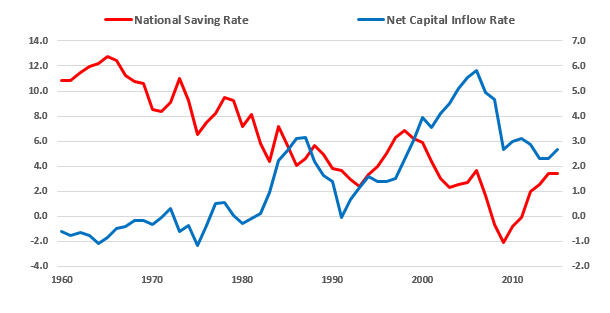
Source: U.S. Bureau of Economic Analysis

In the future, with an aging population collecting Social Security and Medicare benefits, national consumption is projected to increase and national saving to decline. Under current federal tax and expenditures policies, federal deficits are projected to increase in tandem with increased Social Security and Medicare benefit payments. The CBO (Congressional Budget Office: 2016) projects federal debt to increase from 75 percent of GDP today to 86 percent by 2026, and to 141 percent by 2046.

A decline in projected U.S. saving would constrain U.S. domestic investment dollar-for-dollar in a fully closed economy. However, if the economy remains open, foreign capital inflows could offset some of the U.S. saving decline and domestic investment would not decline by as much as the projected decline in U.S. domestic saving. The extent to which foreign saving prevents displacement of U.S. domestic investment depends on continued openness of the economy to trade and capital inflows and the continued willingness of foreign savers to add dollar denominated securities to their asset portfolios.

Foreign Investment Flows: Estimates

Globalization involves increased cross-border trade. The pace of globalization in trade was boosted after World War II until the 2008-09 recession caused a slowdown. This period of rapid globalization was marked by capital account liberalizations, introduction of faster electronic trading systems, better cross-border information exchanges, and declines in transaction costs. Today, despite large trade volumes and faster electronic transfers of liquid capital flows to equalize very short-term after-tax yields on saving, a commensurate increase in cross-border diversification of long-term financial portfolios has not occurred. This “home bias” in long-term financial assets was noted during the early 1980s as a reluctance to diversify financial portfolios across countries and engage in portfolio arbitrage to equalize long-term expected returns (Feldstein and Horoika: 1980). This study finds a strong correlation between domestic saving and investment rates among OECD nations. Although the intensity of home bias appears to have declined over time (Obstfeld and Rogoff: 2000), it still remains high.10

The major reason for a persistent home bias in long term investments appears to be risk aversion. It motivates individual investors to reduce exposure to foreign long-term and illiquid assets regardless of higher expected yields relative to domestic investment opportunities. The return risks are compounded by political uncertainties regarding prospective capital control and tax policies of host countries. Moreover, financial institutions such as mortgage banks, pension funds, and insurance companies may have rules to reduce risk exposures that prevent cross-border portfolio arbitrage to maximize returns. Such individual and institutional rigidities implies that investment demands are inelastic with respect to changes in cross-country in after-tax return differences. A strong and persistent home bias means that domestic investment will be more strongly constrained by domestic saving.11

The U.S. federal government has benefited from financial globalization: U.S. Treasury Department data show that since the year 2000, foreign savers purchased about 40 percent of annual increases in Treasury security issues impelled by higher federal deficits. Thus far during this century, foreign purchases of new government debt has varied between 15 and 60 percent (see Figure 2).

Figure 2: Foreign Take-Up (delta) of Treasury Debt Increases from Previous Year

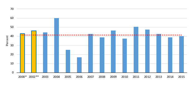
Source: United States Department of the Treasury
*Cumulative delta from 1994;
**Cumulative delta from 2000

As of June 2016, of the $13.9 trillion U.S. treasury debt held by the public, $6.2 trillion (or 44.6 percent) is held in foreign accounts. But U.S. Treasury securities, backed as they are by the full faith and credit of the U.S. federal government, are considered to be among the safest (if not the safest) securities in the world. It’s no wonder that foreign savers are willing to hold almost one-half of outstanding Treasury securities. By contrast, foreign entities (individuals, corporations, and governments) hold only 18.5 percent of total financial securities issued by U.S. domestic sectors including federal, state, and local governments.12

Because foreign savers do not purchase all new issues of Treasury securities, higher projected federal deficits (new Treasury issues) are likely to constrain domestic capital formation. The evidence for this is the fact that foreign official purchases of U.S. government bonds push long-term U.S. interest rates upward (Warnock and Warnock: 1996). This study estimates that with zero foreign inflows into U.S. government bonds, the 10-year Treasury yield would be almost 1 percentage point higher.

The PWBM slider setting spans the range from 0% to 100% to enable users to explore the implications of tax reforms when the economy is fully closed versus fully open to foreign capital inflows, along with two intermediate values of 40% and 70%.

[Updated 11/27/17 to include more detailed discussion about the Frisch elasticity concept. No values have been changed.]

Labor Supply Elasticity (selected bibliography)

Ashenfelter, O. and M. Plant, (1990) “Non-Parametric Estimates of the Labor Supply Effects of Negative Income Tax Programs,” Journal of Labor Economics, vol. 8, pp. 396-415.

Blau, F. and L. Kahn, (2007) “Changes in the Labor Supply Behavior of Married Women: 1980-2000,” Journal of Labor Economics, vol. 25, pp. 393-438.

Chetty, R., J. Friedman and E. Saez, (2013) “Using Differences in Knowledge across Neighborhoods to Uncover the Impacts of the EITC on Earnings,” American Economic Review, vol. 103, no. 7, pp. 2683-2721

Davis, Stephen J., and M. Henrekson, (2005) “Tax Effects on Work Activity, Industry Mix and Shadow Economy Size: Evidence from Rich Country Comparisons,” Labor Supply and Incentives to Work in Europe, R. Gómez-Salvador, A. Lamo, B. Petrongolo, M. Ward, E. Wasmer, eds., pp. 44-104.

Eissa, N. and J. Liebman, (1996) “Labor Supply Response to the Earned Income Tax Credit,” Quarterly Journal of Economics, vol. 111, pp. 605-637.

Gravelle, J., (2014) Dynamic Scoring for Tax Legislation: A Review of Models. Congressional Research Service.

Gruber, Jonathan, and D. A. Wise, (1999) Social Security and Retirement around the World. National Bureau of Economic Research.

Heckman, J. and M. Killingsworth, (1986) “Female Labor Supply: A Survey,” Handbook of Labor Economics, vol. 1, chapter 2.

Munnell, A., (1986) “Lessons from the Income Maintenance Experiments,” Conference Proceedings, Conference Series-30, Federal Reserve Bank of Boston and the Brookings Institution, pp. 1-21.

Pencavel, J., (1986) “Labor Supply of Men: A Survey,” Handbook of Labor Economics, vol. 1, chapter 1.

Pencavel, J., (2002) “A Cohort Analysis of the Association between Work Hours and Wages among Men", Journal of Human Resources, vol. 37, pp. 251-274.

Prescott, Edward C., (2003) “Why Do Americans Work So Much More than Europeans?” Federal Reserve Bank of Minneapolis Research Department Staff Report 321.

Prescott, Edward C., (2006) “Nobel Lecture: The Transformation Macroeconomic Policy and Research.” Journal of Political Economy, vol. 114, no. 2, pp. 203-235.

Rees, A., (1974) “An Overview of the Labor-Supply Results,” Journal of Human Resources, vol. 9, pp. 158-180.

Saez, E., (2010) “Do Taxpayers Bunch at Kink Points?” AEJ: Economic Policy, Vol. 2, pp. 180-212.

Saez, E., J. Slemrod, and S. Giertz, (2012) “The Elasticity of Taxable Income with Respect to Marginal Tax Rates: A Critical Review,"Journal of Economic Literaturevol. 50, quarter 1, pp. 3-50.

Saving Elasticity (selected bibliography)

Attanasio, O. P. and G. Weber (1993), “Consumption Growth, the Interest Rate, and Aggregation,” Review of Economic Studies, vol. 60, no. 3, pp. 631-649.

Avery, Robert B. and A. B. Kennickell (1991), “Household Saving in the U.S.,” Review of Income and Wealth, vol. 37, no. 4, pp. 409-432.

Boskin, M. J. (1978), “Taxation, Saving and the Rate of Interest,” Journal of Political Economy, vol. 86, no. 2, pp. S3-S27.

Bosworth, B. (1984), Tax Incentives and Economic Growth: The Brookings Institution, Washington, D.C.

Bosworth, B., G. Burtless, and J. Sabelhaus (1991) “The Decline in Saving: Evidence from Household Surveys,” Brookings Papers on Economic Activity, Vol. 1, pp. 183-241.

Campbell, John Y., and N. Gregory Mankiw (1989), “Consumption, Income and Interest Rates: Reinterpreting the Time Series Evidence,” in Olivier Jean Blanchard and Stanley Fischer,eds., NBER Macroeconomics Annual: 1989, Cambridge, Mass.: MIT Press, pp. 185-216.

Elmendorf, D. (1996) “The Effect of Interest-rate Changes on Household Saving and Consumption: A Survey,” Board of Governors of the Federal Reserve System (U.S.) in its series Finance and Economics Discussion Series with number 96-27.

Hall, Robert E. (1978), “Stochastic Implications of the Life Cycle - Permanent Income Hypothesis: Theory and Evidence,” Journal of Political Economy, vol. 86, no. 6, pp. 971-987.

Hall, Robert E. (1988), "Intertemporal Substitution in Consumption," Journal of Political Economy, vol. 96, no. 2, pp. 339-357.

Hendershott, P. H. (1990) "Comment," in Joel Slemrod, ed., Do Taxes Matter?: The Impact of the Tax Reform Act of 1986: Cambridge, Mass.: MIT Press.

Skinner, J and D. Feenberg (1990), “The Impact of the 1986 Tax Reform on Personal Saving,” in Joel Slemrod, ed., Do Taxes Matter? The Impact of the Tax Reform Act of 1986, Cambridge, Mass.: MIT Press.

Foreign Investment Flows into U.S. (selected bibliography)

Congressional Budget Office (2016), The 2016 Long Term Budget Outlook, 2016, July.

Feldstein, M. and C. Horoika (1980), “Domestic Saving and International Capital Flows,” The Economic Journal, vol. 90, no. 358, pp. 314-329.

Obstfeld, M. and K. Rogoff (2000), “The Six Major Puzzles in International Macroeconomics: Is There a Common Cause?” Macroeconomics Annual 2000, National Bureau of Economic Research, vol. 15, pp. 339-412.

Warnock, F. E., and V. C. Warnock (2009), “International Capital Flows and U.S. Interest Rates,” Journal of International Money and Finance vol. 28, pp. 903-919.

---

1. Modifications to the framework are considered later in the text. ↩

2. The individual expects not to be alive after next year and consumes positive amounts in both periods. That is “corner outcomes” involving zero consumption this or next year (or choosing extreme poverty in consumption in either of those two years) is precluded.  ↩

3. The interest rate is, therefore, the price of current consumption relative to future consumption. It is assumed that there is no inflation in consumer goods prices between this and next year. It means that the annual interest rate reflects a real price: The trade-off between consumption goods this year and consumption goods next year.  ↩

4. Those wishing to smooth their living standard over time would wish to distribute the wealth increase to consumption in both periods.  ↩

5. Second-period consumption may also decline despite higher saving out of income because of the negative wealth effect.  ↩

6. A higher interest rate may reduce the amount of desired borrowing for funding current consumption, but not by enough to eliminate it.  ↩

7. A simplifying feature of such models is that corporate undistributed profits can be directly attributed to household decisions.  ↩

8. The measurement of long-term saving elasticity involves too many additional complicating factors.  ↩

9. See the Public Policy Initiative Brief: Not Enough Shovels: The Crucial Role of Future Capital Accumulation for U.S. Output Growth.  ↩

10. Across OECD countries, the correlation between saving and investment rates out of income declined from 0.89 during the sixties and seventies, to 0.60 during the 1990s.  ↩

11. A similar home bias in intranational (cross-regional) capital flows is not supported by empirical evidence (Obstfeld and Rogoff: 2001).  ↩

12. Data from the U.S. Department of the Treasury available at: http://ticdata.treasury.gov/Publish/slt3d.txt and http://www.treasurydirect.gov/govt/reports/pd/mspd/2016/opds062016.pdf. In comparison, foreigners hold about 18.5 percent of total financial securities issued by U.S. domestic sectors including federal, state, and local governments. See Flow of Funds Matrix provided by the Board of Governors of the U.S. Federal Reserve System, available at: https://www.federalreserve.gov/releases/z1/current/z1.pdf.  ↩